Otros

Resumen

Una visualización de datos correcta puede expresar de forma resumida y clara gran cantidad de información, ayudando a interpretar y asimilar la información más facilmente.

———–

Gráfico de mosaico

Código

library(vcd)

Código

mosaic(~ Class + Survived, data = Titanic, shade = TRUE, legend = TRUE)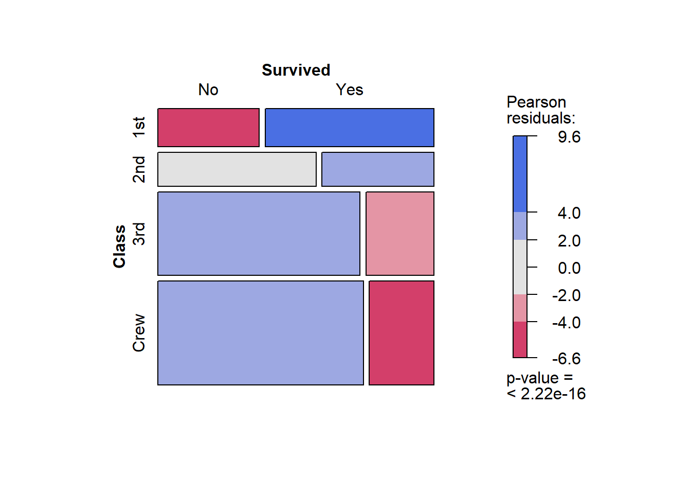

Código

library(ggplot2)
library(dplyr)

Código

# Crear un marco de datos con categorías
data <- data.frame(
  Categoria1 = rep(c("A", "B", "C"), each = 3),
  Categoria2 = rep(c("X", "Y", "Z"), times = 3),
  Count = c(10, 20, 30, 5, 15, 25, 20, 10, 5)
)

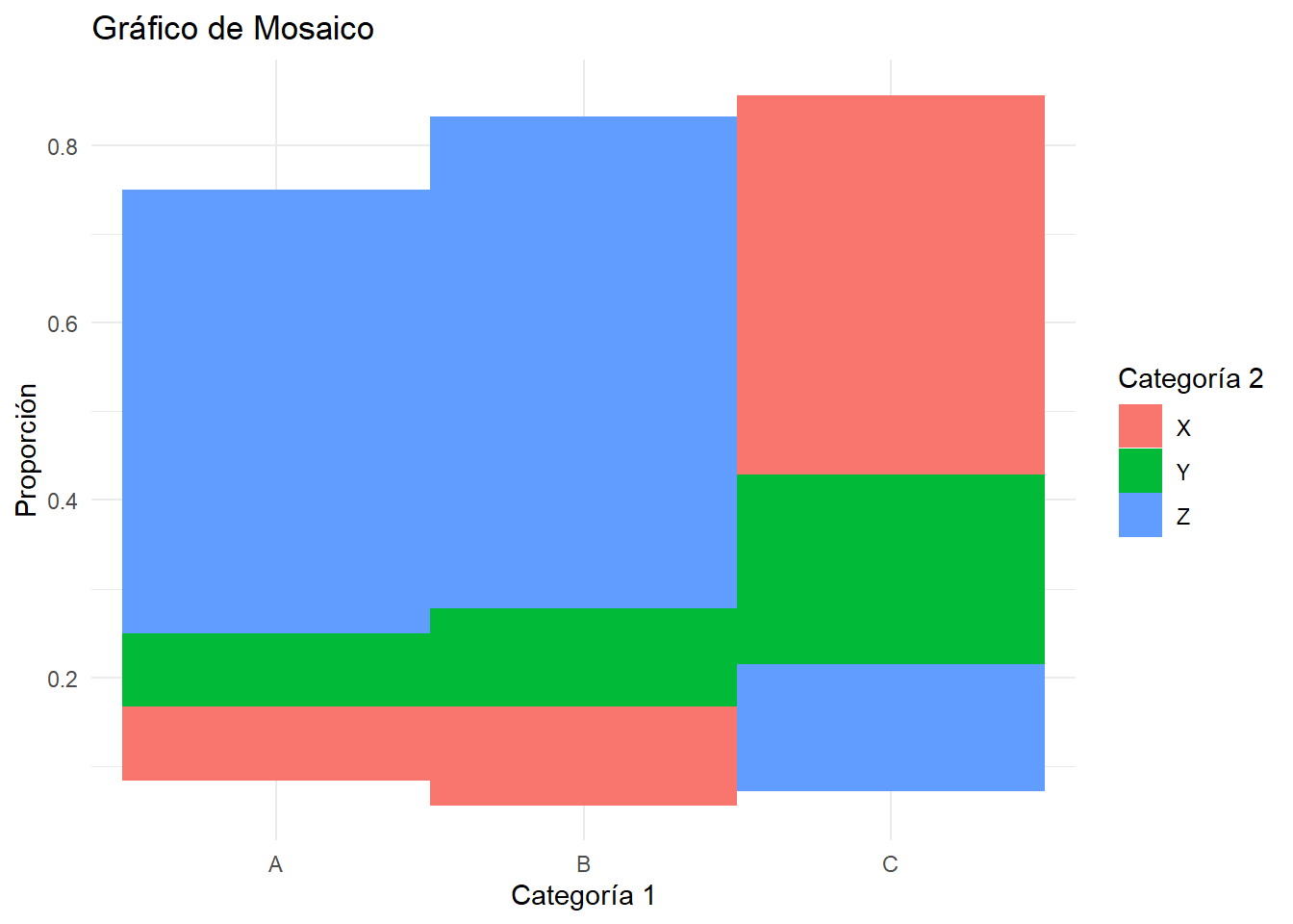
# Calcular proporciones
data <- data %>%
  group_by(Categoria1) %>%
  mutate(Proporcion = Count / sum(Count)) %>%
  ungroup()

# Crear el gráfico de mosaico
ggplot(data, aes(x = Categoria1, y = Count, fill = Categoria2)) +
  geom_tile(aes(height = Count)) +
  labs(title = "Gráfico de Mosaico",
       x = "Categoría 1",
       y = "Proporción",
       fill = "Categoría 2") +
  theme_minimal()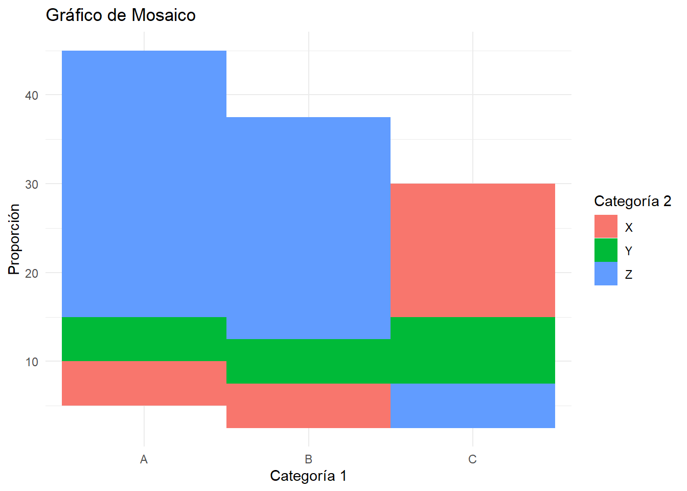

Código

# Crear el gráfico de mosaico
ggplot(data, aes(x = Categoria1, y = Proporcion, fill = Categoria2)) +
  geom_tile(aes(height = Proporcion)) +
  labs(title = "Gráfico de Mosaico",
       x = "Categoría 1",
       y = "Proporción",
       fill = "Categoría 2") +
  theme_minimal()

Código

#ggplot(data = fly) +
#  geom_mosaic(aes(x=product(do_you_recline), fill = do_you_recline, 
#                  conds = product(rude_to_recline))) +
#  labs(title='f(do_you_recline | rude_to_recline)')

Mapa de calor iteractivo

Código

# Librerías
library(ggplot2)
library(reshape2)
library(heatmaply)

# Datos
data <- cor(mtcars)

# Mapa de calor
heatmaply(data, k_row = 3, k_col = 2, main = "Correlación entre variables de mtcars")

Tree map

Código

# Librerías
library(ggplot2)
library(treemapify)

# Datos
data <- data.frame(
  category = c("A", "B", "C", "D"),
  value = c(40, 30, 20, 10)
)

# Gráfico de árbol
ggplot(data, aes(area = value, fill = category, label = category)) +
  geom_treemap() +
  geom_treemap_text(colour = "white", place = "centre") +
  labs(title = "Distribución de categorías")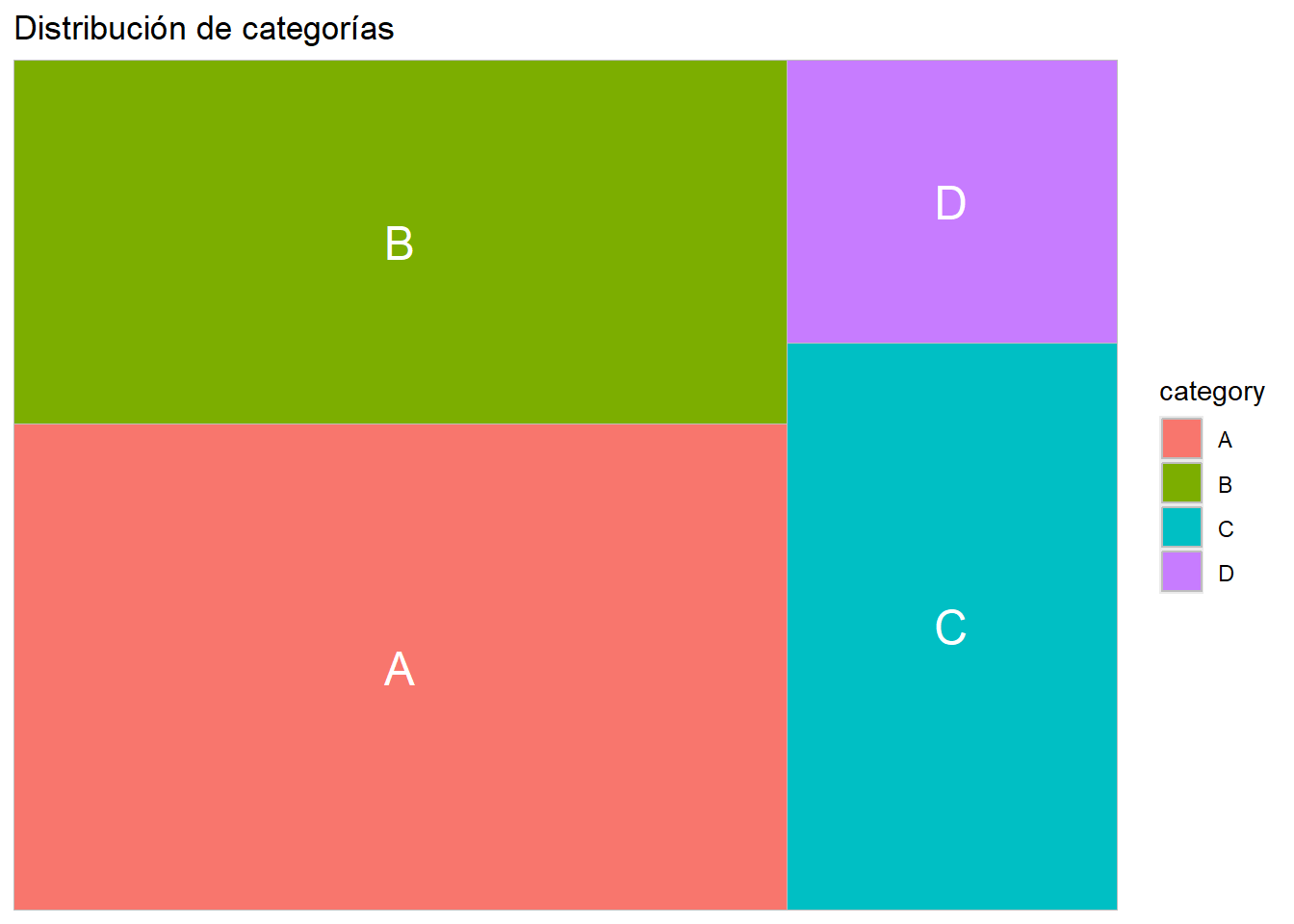

Mapa coroplético

Código

# Librerías
library(ggplot2)
library(maps)

# Datos
data <- map_data("state")
data$rate <- runif(nrow(data), min = 0, max = 1)

# Mapa coroplético
ggplot(data, aes(long, lat, group = group)) +
  geom_polygon(aes(fill = rate), color = "white") +
  scale_fill_continuous(low = "white", high = "blue") +
  labs(title = "Tasa aleatoria por estado")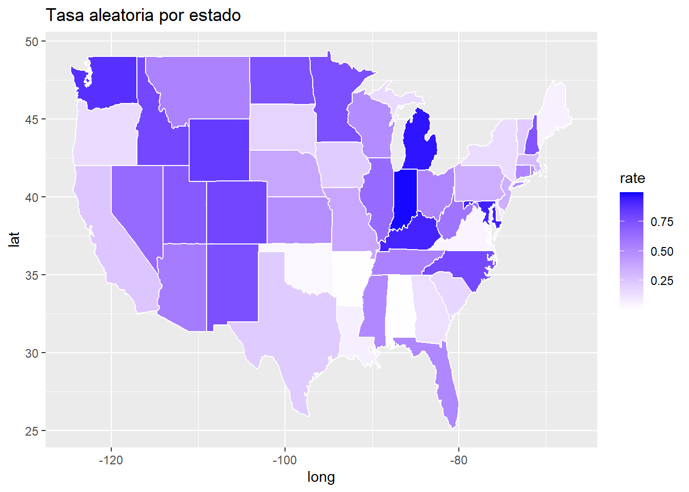

Gráfico de Sankey

Código

# Librerías
library(networkD3)

# Datos
nodes <- data.frame(name = c("A", "B", "C", "D"))
links <- data.frame(
  source = c(0, 1, 1, 2, 3),
  target = c(1, 2, 3, 3, 2),
  value = c(10, 20, 30, 40, 50)
)

# Gráfico de Sankey
sankeyNetwork(Links = links, Nodes = nodes, Source = "source", Target = "target",
              Value = "value", NodeID = "name", fontSize = 12)

Código

# Librerías
library(fmsb)

# Datos
data <- as.data.frame(matrix(sample(2:20, 10, replace = TRUE), ncol = 5))
colnames(data) <- c("A", "B", "C", "D", "E")

# Gráfico de radar
# radarchart(data, axistype = 1, pcol = "blue", pfcol = scales::alpha("blue", 0.5))

Código

## 11. Gráfico de Radar o Araña

# Librerías
library(fmsb)

# Datos
data <- data.frame(
  A = c(10, 15, 8),
  B = c(9, 17, 6),
  C = c(12, 13, 9),
  D = c(8, 10, 14),
  E = c(15, 8, 12)
)

# Agregar las filas máximas y mínimas para escalar el gráfico
data <- rbind(rep(20, 5), rep(0, 5), data)

# Gráfico de radar
radarchart(data, axistype = 1, 
           pcol = rainbow(3), 
           pfcol = scales::alpha(rainbow(3), 0.4), 
           plwd = 2, 
           cglcol = "grey", 
           cglty = 1, 
           axislabcol = "grey", 
           caxislabels = seq(0, 20, 5), 
           cglwd = 0.8)

Gráfico de Mariposa (Population Pyramid)

Código

# Librerías
library(ggplot2)

# Datos
data <- data.frame(
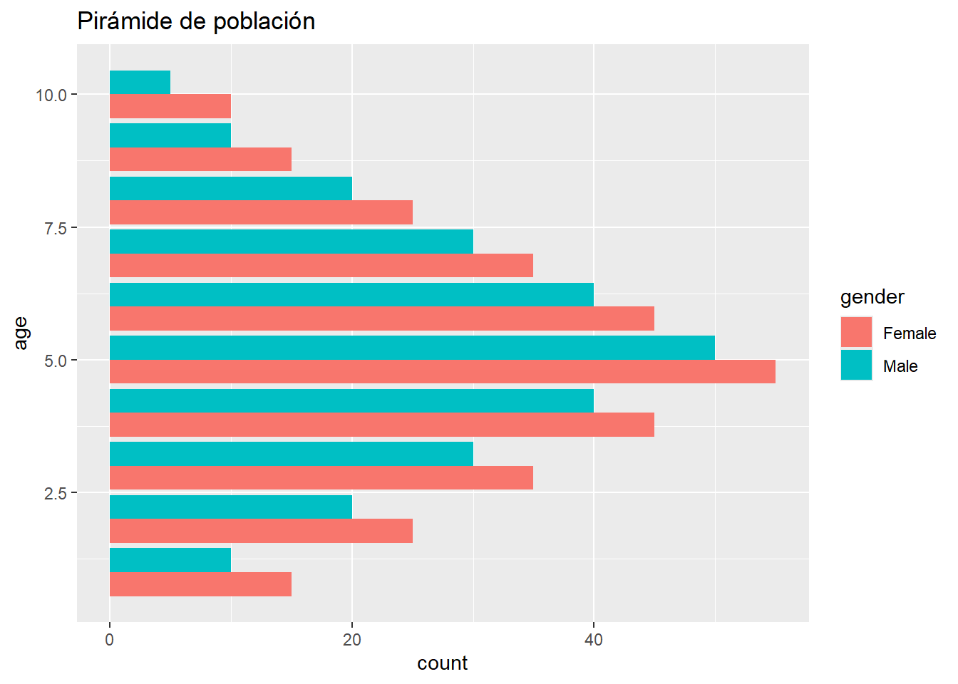
  age = rep(1:10, 2),
  count = c(10, 20, 30, 40, 50, 40, 30, 20, 10, 5, 15, 25, 35, 45, 55, 45, 35, 25, 15, 10),
  gender = rep(c("Male", "Female"), each = 10)
)

# Gráfico de mariposa
ggplot(data, aes(x = age, y = count, fill = gender)) +
  geom_bar(stat = "identity", position = "dodge") +
  coord_flip() +
  labs(title = "Pirámide de población")

Gráfico de burbujas

Código

# Librerías
library(ggplot2)

# Datos
data <- data.frame(
  x = rnorm(100),
  y = rnorm(100),
  size = rnorm(100, mean = 5, sd = 2)
)

# Gráfico de burbujas
ggplot(data, aes(x = x, y = y, size = size)) +
  geom_point(alpha = 0.5) +
  labs(title = "Gráfico de burbujas")