Ejercicio 1
Un investigador dispone de los siguientes datos de un conjunto de pacientes con enfermedad pulmonar que necesitan un trasplante de pulmón. La variable principal es el tiempo (time), en días, hasta que el paciente recibe el trasplante de pulmón; además se dispone de la siguiente información.
status: 0 censurado, 1 trasplante.
age: edad del paciente
gender: 1 mujer, 2 hombre.
bmi: IMC numérico.
disease: estadio de la enfermedad (1,2,3).
past: antecedentes familiares de enfermedad pulmonar (0 no, 1 sí)
Realizar una estimación de la función de supervivencia sin utilizar ninguna de las covariables. Obtener el valor de la mediana de seguimiento y la supervivencia a los 147 días.
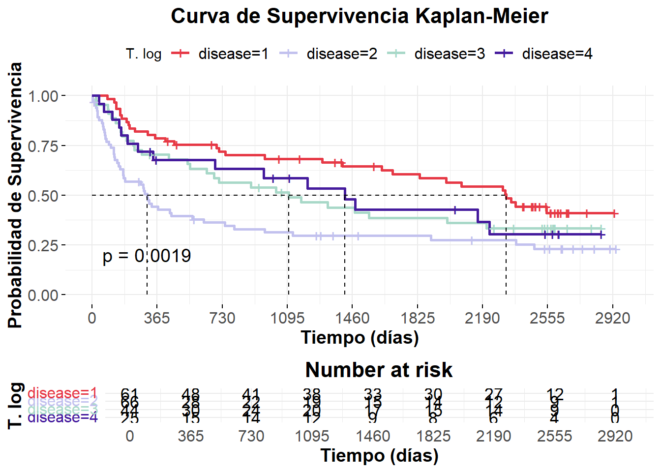
Comparar la supervivencia en función de cada covariable categórica.
Tiempo hasta el evento AKA trasplante: ¿tiempo supervivencia global (overall survival) o tiempo hasta enfermedad progresiva (time to progressive disease)? Yo creo que la segunda.
Lectura de datos.
ejercicio2 <- haven::read_dta("~/Master_Bioestadistica/Supervivencia/Tema_02/Datos Ejercicio 2/lung_transplant.dta")
ejercicio2 |> dim(); summary(ejercicio2)
## [1] 196   8
##     patient            time            status            age
##  Min.   :  1.00   Min.   :   3.0   Min.   :0.0000   Min.   :18.00
##  1st Qu.: 49.75   1st Qu.: 182.2   1st Qu.:0.0000   1st Qu.:41.75
##  Median : 98.50   Median : 843.5   Median :1.0000   Median :53.00
##  Mean   : 98.50   Mean   :1182.2   Mean   :0.6276   Mean   :48.56
##  3rd Qu.:147.25   3rd Qu.:2387.5   3rd Qu.:1.0000   3rd Qu.:58.00
##  Max.   :196.00   Max.   :2939.0   Max.   :1.0000   Max.   :67.00
##      gender           bmi           disease           past
##  Min.   :1.000   Min.   :14.00   Min.   :1.000   Min.   :0.0000
##  1st Qu.:1.000   1st Qu.:19.50   1st Qu.:1.000   1st Qu.:0.0000
##  Median :1.000   Median :22.60   Median :2.000   Median :0.0000
##  Mean   :1.429   Mean   :23.42   Mean   :2.168   Mean   :0.3418
##  3rd Qu.:2.000   3rd Qu.:27.52   3rd Qu.:3.000   3rd Qu.:1.0000
##  Max.   :2.000   Max.   :35.20   Max.   :4.000   Max.   :1.0000
status: 0 censurado, 1 trasplante status: 37.24 % censurado, 62.76 % trasplante
¿median(time) = 843.5? ¡No…!
head(ejercicio2)
## # A tibble: 6 × 8
##   patient  time status   age gender   bmi disease  past
##     <dbl> <dbl>  <dbl> <dbl>  <dbl> <dbl>   <dbl> <dbl>
## 1       1  2324      1    59      1  29.6       1     0
## 2       2   108      1    28      1  22.6       3     0
## 3       3  2939      0    55      1  32.1       2     1
## 4       4  1258      0    62      1  30         2     1
## 5       5  2904      0    51      1  30.4       2     1
## 6 6 444 1 59 1 26.9 2 1ggplot(ejercicio2, aes(x = time)) +
geom_histogram(bins = 100) +
geom_vline(xintercept = seq(365, max(ejercicio2$time), by = 365),
linetype = "dashed", color = "lightblue") +
scale_x_continuous(breaks = seq(0, max(ejercicio2$time), by = 365),
labels = paste0("Año ", seq(0, max(ejercicio2$time) / 365))) +
labs(title = "Distribución time", x = "time (días)", y = "freq.") +
theme_minimal() +
theme(panel.grid = element_blank(),
axis.text.x = element_text(color = "blue"))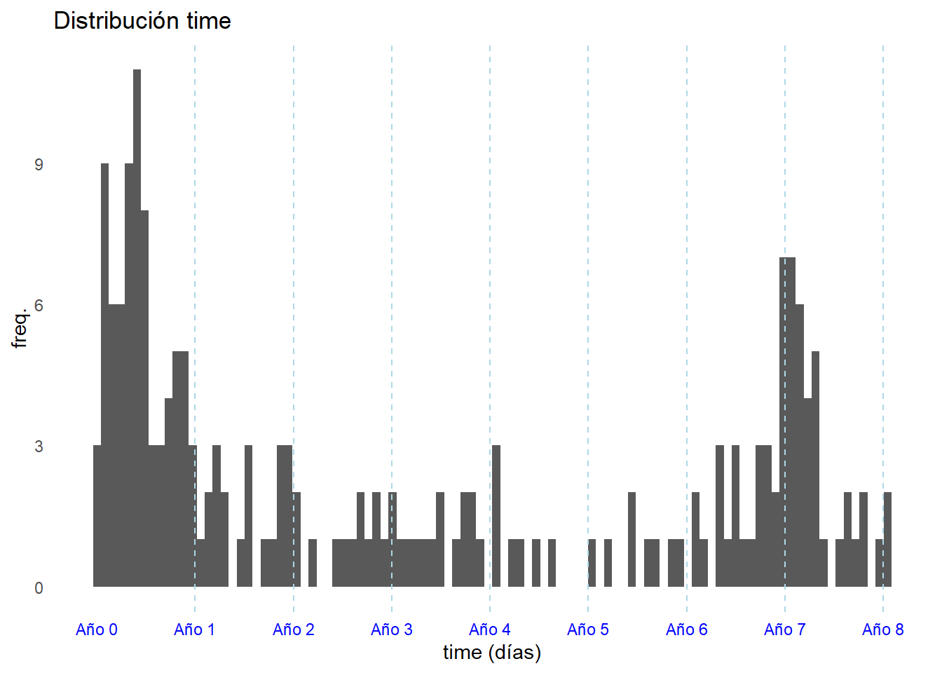
ggplot(ejercicio2, aes(x = time / 30)) +
  geom_histogram(bins = 40) +
  geom_vline(xintercept = seq(12, max(ejercicio2$time / 30), by = 12),
             linetype = "dashed", color = "lightblue") +
  scale_x_continuous(breaks = seq(0, max(ejercicio2$time / 30), by = 12),
                     labels = paste0("Año ", seq(0, max(ejercicio2$time / 30) / 12))) +
  labs(title = "Distribución time", x = "time (meses)", y = "freq.") +
  theme_minimal() +
  theme(panel.grid = element_blank(),
        axis.text.x = element_text(color = "blue"))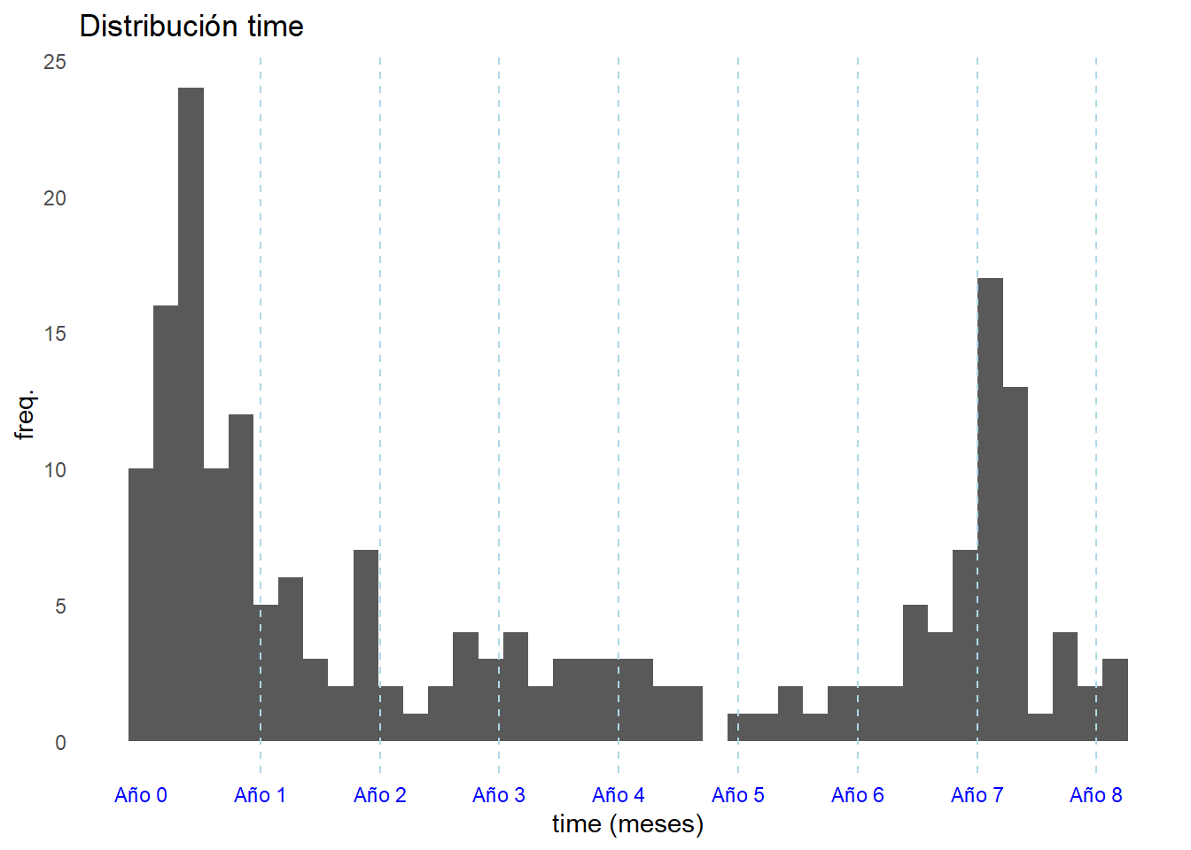
Surv(time, status == 0)
- Surv() crea un objeto de supervivencia.
- time: variable que indica el tiempo hasta el evento o censura.
- status == 0: define que el evento de interés ocurre cuando status == 1 (considera 1 el evento).
La mayoría de los censurados son para valores de tiempo más altos. Posiblemente estas censuras sean porque se cerró el estudio.
  [1]    3     4    11+   16    21    22    25    29    31    31    38    38
 [13]   55    61    63    65    70    73    76    80    85    88    92    95
 [25]  104   108   114   121   121   123   124   128   132   134   136   142
 [37]  148   151   153   158   158   158   159   162   165   169   174   175
 [49]  177   184   192   192   199   203   209   231   237   239   257   263+
 [61]  273   278   288   290   294   310   311   313   320   322+  326+  335
 [73]  343   354   358+  371   410   425+  431   437   444   461   474+  535
 [85]  549   563   571+  625   642   671+  683   689   697   711   711   744
 [97]  749   797   890   934+  962   967   969  1015+ 1032  1049+ 1062+ 1104
[109] 1105+ 1125  1165+ 1173  1208  1258+ 1283+ 1290  1321  1353+ 1364+ 1400+
[121] 1405  1419  1474  1477  1493+ 1553  1581+ 1624  1686  1836  1901  1987
[133] 1991  2037+ 2071  2131+ 2162  2212  2230  2254+ 2303  2317  2324  2349
[145] 2364+ 2375  2378  2416+ 2421+ 2466+ 2471+ 2473+ 2479  2485+ 2487+ 2510+
[157] 2523+ 2538+ 2538+ 2542+ 2545+ 2550  2555+ 2565+ 2571+ 2573+ 2575+ 2582+
[169] 2586+ 2586+ 2591+ 2596+ 2596+ 2612+ 2616+ 2616+ 2618+ 2628+ 2631+ 2636+
[181] 2638+ 2661+ 2664+ 2670+ 2671+ 2672+ 2699+ 2751+ 2775+ 2801+ 2817+ 2854+
[193] 2856+ 2904+ 2929+ 2939+Call: survfit(formula = with(ejercicio2, Surv(time, status)) ~ 1)
n events median 0.95LCL 0.95UCL
[1,] 196 123 1125 697 1901KM1_log <- survfit(with(ejercicio2, Surv(time, status) ~ 1, conf.type='log')) # IC de transformación log (BY DEFAULT)
KM1_log # Curva de supervivenciaCall: survfit(formula = with(ejercicio2, Surv(time, status) ~ 1, conf.type = "log"))
n events median 0.95LCL 0.95UCL
[1,] 196 123 1125 697 1901¡median(time) = 1125! (697, 1901)
Día en el cual el 50 % de los individuos de la cohorte han tenido un trasplante. Indica el punto en el cual la probabilidad de que un individuo no tenga el trasplante es del 50 %.
KM1_plain <- survfit(with(ejercicio2, Surv(time, status) ~ 1, conf.type='plain')) # IC de la aprox normal
KM1_plain # Curva de supervivencia
Call: survfit(formula = with(ejercicio2, Surv(time, status) ~ 1, conf.type = "plain"))
n events median 0.95LCL 0.95UCL
[1,] 196 123 1125 697 1901KM1_loglog <- survfit(with(ejercicio2, Surv(time, status) ~ 1, conf.type='log-log')) # IC de transformación log-log
KM1_loglog # Curva de supervivencia Call: survfit(formula = with(ejercicio2, Surv(time, status) ~ 1, conf.type = "log-log"))
n events median 0.95LCL 0.95UCL
[1,] 196 123 1125 697 1901survminer::ggsurvplot(KM1_log,
data = ejercicio2,
title = "Curva de supervivencia",
subtitle = '(by ggsurvplot)',
conf.int = T,
surv.median.line = "hv") # líneas H y V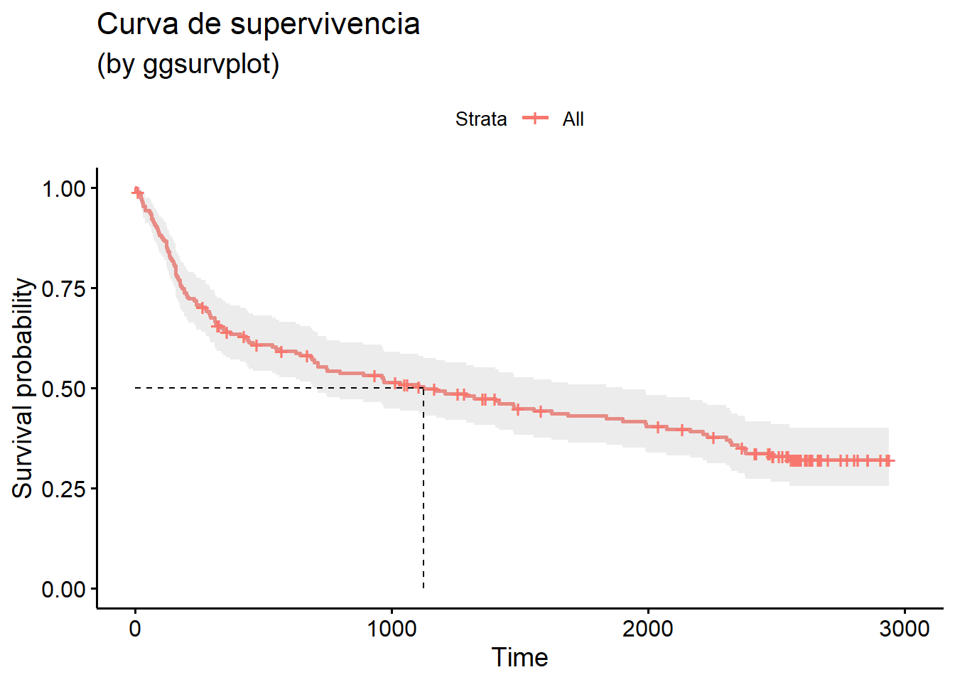
prodlim::Hist proporciona las extensiones adecuadas para tratar con datos censurados a la derecha y censurados por intervalos de riesgos competitivos y otros modelos multiestado.
prodlim::Hist(ejercicio2$time, ejercicio2$status)
Right-censored response of a survival model

No.Observations: 196

Pattern:
                Freq
 event          123
right.censored 73 Quantiles of the event time distribution based on the Kaplan-Meier method.
Table of quantiles and corresponding confidence limits:
q quantile lower upper
<num> <num> <num> <num>
1: 0.00 NA NA NA
2: 0.25 NA 2550 NA
3: 0.50 1125 697 1836
4: 0.75 184 153 290
5: 1.00 3 3 21
Median with interquartile range (IQR):
Median (IQR)
<char>
1: 1125.00 (184.00;NA)¡median(time) = 1125! (697, 1836). Antes (697, 1901)
Código
survminer::ggsurvplot(
  KM1_log,
  data = ejercicio2,
  conf.int = TRUE,                      # Intervalos de confianza
  conf.int.style = "ribbon",            # Sombreado para el IC
  break.time.by = 365,                    # Ejes en intervalos de 5
  risk.table = TRUE,                     # Tabla de riesgo debajo
  risk.table.height = 0.25,              # Tamaño de la tabla de riesgo
  risk.table.col = "black",              # Color del texto de la tabla de riesgo
  pval = TRUE,                           # Mostrar p-valor
  surv.median.line = "hv",               # Línea en la mediana de supervivencia
  legend.title = "T. log",   # Título de la leyenda
  legend.labs = c("Supervivencia Global"), # Etiqueta de la leyenda
  palette = c("#E63946"),                # Color principal de la curva
  xlab = "Tiempo (días)",                # Etiqueta del eje X
  ylab = "Probabilidad de Supervivencia",# Etiqueta del eje Y
  title = "Curva de Supervivencia Kaplan-Meier", # Título principal
  ggtheme = theme_minimal() +             # Estilo de la gráfica
    theme(
      plot.title = element_text(hjust = 0.5, size = 16, face = "bold"),
      axis.title = element_text(size = 14, face = "bold"),
      axis.text = element_text(size = 12),
      legend.position = "bottom",
      legend.text = element_text(size = 12)
    )
)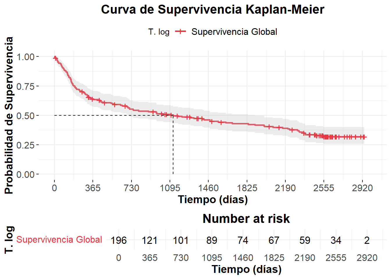
Supervivencia a los 147 días: 0.821 (0.768, 0.876).
summary(KM1_log, time = 147, extend = TRUE) Call: survfit(formula = with(ejercicio2, Surv(time, status) ~ 1, conf.type = "log"))
time n.risk n.event survival std.err lower 95% CI upper 95% CI
147 160 35 0.821 0.0275 0.768 0.876KM2_log <- survfit(with(ejercicio2, Surv(time, status) ~ disease , conf.type='log')) # IC de transformación log (BY DEFAULT)
KM2_log # Curva de supervivenciaCall: survfit(formula = with(ejercicio2, Surv(time, status) ~ disease,
conf.type = "log"))
n events median 0.95LCL 0.95UCL
disease=1 61 32 2324 1686 NA
disease=2 66 48 310 175 744
disease=3 44 28 1104 642 NA
disease=4 25 15 1419 689 NACódigo
survminer::ggsurvplot(
  KM2_log,
  data = ejercicio2,
  conf.int = FALSE,                      # Intervalos de confianza
  conf.int.style = "ribbon",            # Sombreado para el IC
  break.time.by = 365,                    # Ejes en intervalos de 5
  risk.table = TRUE,                     # Tabla de riesgo debajo
  risk.table.height = 0.25,              # Tamaño de la tabla de riesgo
  risk.table.col = "black",              # Color del texto de la tabla de riesgo
  pval = TRUE,                           # Mostrar p-valor
  surv.median.line = "hv",               # Línea en la mediana de supervivencia
  legend.title = "T. log",   # Título de la leyenda
  legend.labs = c("disease=1","disease=2","disease=3","disease=4"), # Etiqueta de la leyenda
  palette = c("#E63946", "#c2c1Ee", "#A8d8c8", "#451b9D"),                # Color principal de la curva
  xlab = "Tiempo (días)",                # Etiqueta del eje X
  ylab = "Probabilidad de Supervivencia",# Etiqueta del eje Y
  title = "Curva de Supervivencia Kaplan-Meier", # Título principal
  ggtheme = theme_minimal() +             # Estilo de la gráfica
    theme(
      plot.title = element_text(hjust = 0.5, size = 16, face = "bold"),
      axis.title = element_text(size = 14, face = "bold"),
      axis.text = element_text(size = 12),
      legend.position = "bottom",
      legend.text = element_text(size = 12)
    )
)